Simple Poisson Solver
Introduction
What, why?
If you were unlucky enough to be subjected to an undergraduate physics or mathematics course then you will have probably stumbled into the interesting world of partial differential equations (PDEs) where you might have discovered the excellent toolkit we use to model systems that change over space and time. There are many types of PDEs I will give a little background on these for the reader who was lucky enough to avoid them:
- linear/non-linear (1st order PDE) - I always use basic resistive-capacitive or resistive-inductive circuits as an example of some linear 1st order PDEs, however if you aren’t into circuit theory then LibreText Mathematics has a good example which is modelling a rock that is being carried down a river (okay we are assuming the rock doesnt diffuse into the surrounding water as if it was loose sediment). An example of a non-linear 1st order PDE is the invicid burgers’ equation which is used to model shocks and not sandwhiches.
- parabolic (2nd order PDE)
- hyperbolic (2nd order PDE)
- elliptical (2nd order PDE)
- higher order PDEs probably - I am no mathematician sadly
PDEs. A great example of these are Laplace’s Equation and the more general expression Poisson’s Equation. These are elliptical PDEs
One of most basic equations we can work with is \( \nabla^2\phi = \frac{\rho}{\varepsilon_0} \)
Let’s start solving some PDEs
Gauss-Seidel Method
Otherwise known as the method of successive displacement. This is an iterative method for determining the solution to our PDE, all this means is that we start with some estimate of the solution \( \phi_0 \) which is improved upon the successive application of some iterative process. I am going to go into a little more detail about this method, and the mathematics of it, however if you only want to see the implementation and performance then feel free to skip this part.
Discretising our problem
As we are working in the realm of numerical solvers the first step is to properly discretise our equations so lets look at solving Poissons Equation in 2D where we have an arbitrary source term \( f(x,y) \) on a cartesian grid
\[ \nabla^2 \phi = \partial^2_x \phi(x,y) + \partial^2_y \phi(x,y) = f(x,y) \]
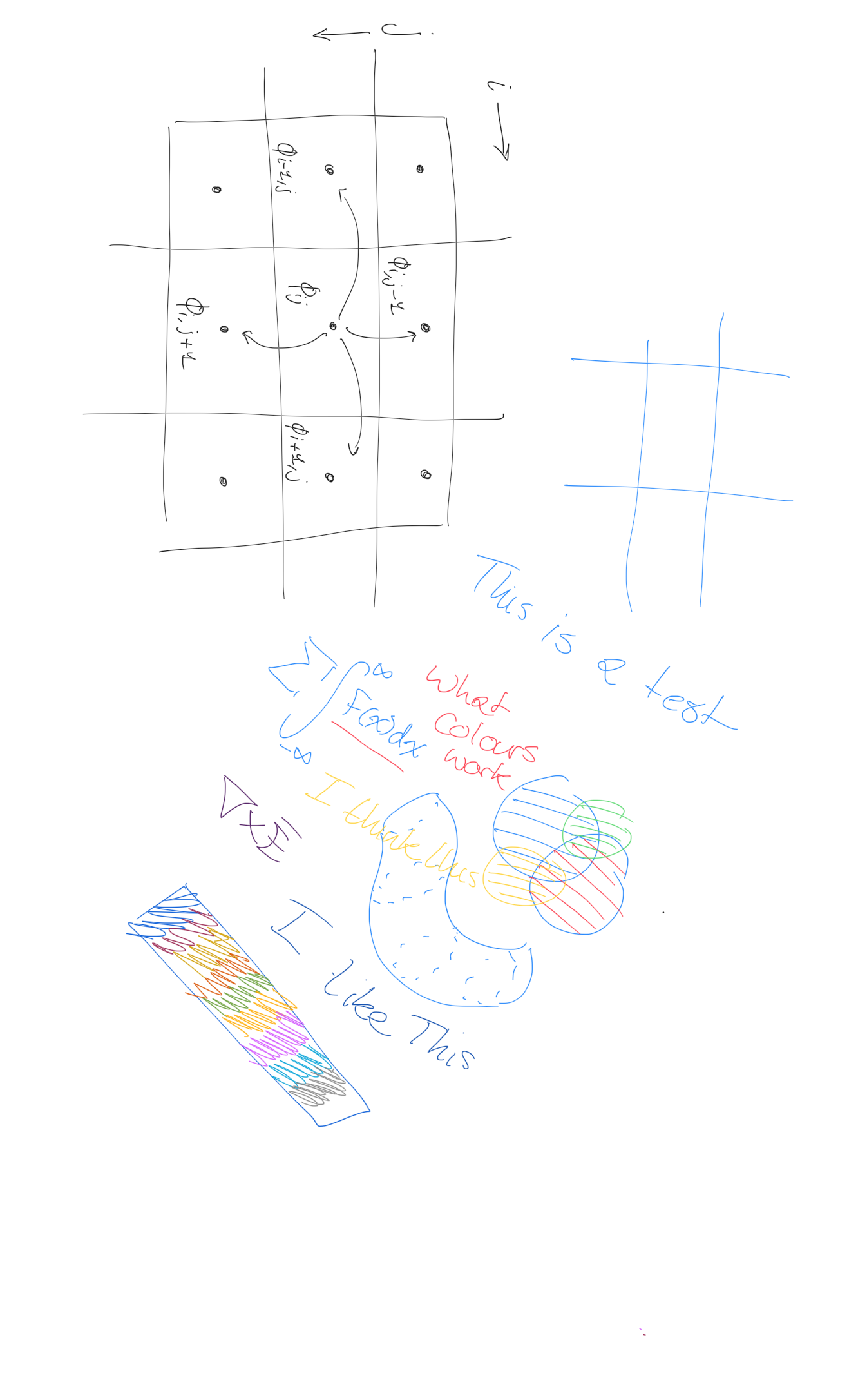
Now before we try solving this lets formulate a nice way to do this. So first lets get our useful term, \( \partial^2 \phi \) using the taylor series expansion for a central difference approximation of the derivative. We can do this if we imagine our grid and the derivative at point \( \phi_{i,j} \) is what we want to find so we must look at the surrounding grid cells and create an expression for these \( \phi_{i\pm 1,j\pm 1} \), we can do this via a taylor expansion as [SOMETHING] and, I will just show this for i but the same is true for the verticle index j, this is expressed as
\[ \phi_{i+1} = \phi_i + \frac{d\phi}{dx}h + \frac{d^2\phi}{dx^2}\frac{h^2}{2!} + … + O(h_x^2) \]
\[ \phi_{i-1} = \phi_i - \frac{d\phi}{dx}h + \frac{d^2\phi}{dx^2}\frac{h^2}{2!} + … + O(h_x^2) \]
and now we can see a nice \( \frac{d^2\phi}{dx^2}\) which is exactly what we want so we can rearrange both of these equation to get
\[ \phi_{i+1} + \phi_{i-1} = 2\phi_i + \frac{d^2\phi}{dx^2}h^2 + O(h_x^2) \]
\[ \frac{d^2\phi}{dx^2} = \frac{\phi_{i-1}+2\phi_{i}+\phi_{i+1}}{h_x^2} = f(x)\]
and now we are getting somewhere, the keen reader will see that our second derivative can be calculated purely by relying on the surrounding values! That is great. So lets do this with \( j \) and we now should be able to find \( \partial^2\phi(x,y) \) and lets also assume \( h^2\)
\[ {\phi_{i-1,j} + \phi_{i+1,j}} + {\phi_{i,j-1} + \phi_{i,j+1}}+ 4\phi_{i,j} - f(x,y)(h^2)\]
This is a form of the 5-point stencil for the Laplacian! And as a note this is also true for finite volume method (FVM) if we integrate \( \nabla^2 \phi = f\) over some control volume and apply Gauss’ theorem then we get the flux flowing though the faces. And if we have an uniform othogonal mesh, then this can still be expressed as a weighted average of the neighbours, if we had a non othogonal grid, then we would have a coefficient change but we can still performan the iterative process. When working with the more common finite element method (FEM) we can get a sparse matrix (this is just a matrix that represents our system of equations) it usually looks something like \( \mathbf{A} \phi = b\)
Red Black Gauss-Seidel Method
A nice optimisation of our gauss-seidel method is to use the “Red Black” method where we color our central node \( \phi_{i,j} \) as red and its four neighbours as black, this means that when we are solving our solution all our red nodes only depend on black nodes and all our black nodes depend only on red nodes. Extending this to FVM and FEM is also possible however we might need to introduce multiple colors rather than just two which we can do using some graph coloring algorithm.